Points

The simplest thing the panel draws, and the one that needs the least from your query: two coordinate columns, and everything else is optional.

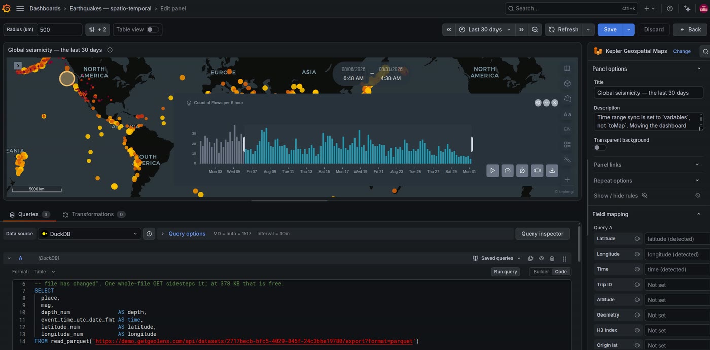
The minimum

SELECT lat AS latitude,
       lon AS longitude
FROM gps_readings;

The map frames itself on the data and kepler builds a Point layer.

Points are small by default

kepler's default radius is deliberately modest, and on a country-sized view a few thousand points can read as nothing at all. If the map looks empty but the query returned rows, raise Radius in the layer panel before concluding that detection failed.

The column names that are recognised

Matched case-insensitively and exactly:

Role	Names
Latitude	latitude, lat, y
Longitude	longitude, lon, lng, long, x

x and y are in the list because a lot of tables use them, but note that they are matched as degrees, not as projected coordinates — the panel renders WGS84 (EPSG:4326) only and does not reproject. A table of UTM eastings and northings called x/y will be detected and will land in the Gulf of Guinea.

Anything else — pos_lat, punto_latitud, lat_wgs84 — is not detected, and is mapped by hand under Field mapping. That is a per-query setting, so two queries in one panel can use different conventions.

Everything else in the row comes with it

Columns without a role are passed through untouched, which is what makes them useful:

SELECT lat  AS latitude,
       lon  AS longitude,
       recorded_at,          -- detected as time, by type
       speed_kmh,            -- colour scale, size, filter, tooltip
       vehicle_type,         -- category colour, filter
       driver_name           -- tooltip
FROM gps_readings;

In kepler's layer panel those become Color Based On and Radius Based On options, filter targets, and tooltip fields. Nothing is dropped for not having a role.

Time

A time column is detected by type rather than by name, because Grafana already knows which column is temporal and dashboards call it anything. Whatever your time column is called, if the data source typed it as time, it is found.

What a time column buys you:

• A time filter in kepler's filter panel, with a histogram and a brush.
• Coupling to the dashboard time picker — see Time range sync.
• Playback, when combined with a trip id — see Trajectories.

If your time arrives as an epoch integer or a string, cast it in the query so the data source types it as a timestamp; a numeric column will otherwise be treated as an ordinary measure.

kepler's own convention also works

Detection runs on two levels. Above the panel's own roles, kepler applies its own column-name conventions to whatever it receives — and one of them is a <prefix>_lat + <prefix>_lng pair.

So a CSV whose columns are point_latitude and point_longitude produces a point layer even though neither name is in the table above: the panel does not claim them, and kepler recognises the pair. This is worth knowing mostly so that an unexpected extra layer makes sense when you see one.

Volume

Points are the cheapest layer there is, and deck.gl will draw a great many of them. The constraint is usually not rendering but transport: every row travels from the data source through Grafana into the browser as JSON. Tens of thousands is comfortable, hundreds of thousands is noticeable, and past that you want to aggregate in SQL or switch to a layer that aggregates for you — grid, hexbin, heatmap or cluster, all of which are in the layer gallery.

When it is not points you want

• Rows have a geometry column rather than a coordinate pair → Geometry
• Rows have a vehicle or trip id and a time → Trajectories
• Rows are an origin and a destination → Origin–destination flows
• Rows are a hexagon or cell identifier → H3 and S2
• Rows are a grid of velocities → Wind and other velocity fields